Background
Statistical Machine Translation as a research area started in the late 1980s with the Candide project at IBM. IBM's original approach maps individual words to words and allows for deletion and insertion of words.
Lately, various researchers have shown better translation quality with the use of phrase translation. Phrase-based MT can be traced back to Och's alignment template model, which can be re-framed as a phrase translation system. Other researchers used augmented their systems with phrase translation, such as Yamada, who use phrase translation in a syntax-based model.
Marcu introduced a joint-probability model for phrase translation. At this point, most competitive statistical machine translation systems use phrase translation, such as the CMU, IBM, ISI, and Google systems, to name just a few. Phrase-based systems came out ahead at a recent international machine translation competition (DARPA TIDES Machine Translation Evaluation 2003-2006 on Chinese-English and Arabic-English).
Of course, there are other ways to do machine translation. Most commercial systems use transfer rules and a rich translation lexicon. Machine translation research was focused on transfer-based systems in the 1980s and on knowledge based systems that use an interlingua representation as an intermediate step between input and output in the 1990s.
There are also other ways to do statistical machine translation. There is some effort in building syntax-based models that either use real syntax trees generated by syntactic parsers, or tree transfer methods motivated by syntactic reordering patterns.
The phrase-based statistical machine translation model we present here was defined by Koehn et al. (2003). See also the description by Zens (2002). The alternative phrase-based methods differ in the way the phrase translation table is created, which we discuss in detail below.
Model
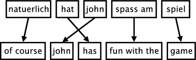
The figure below illustrates the process of phrase-based translation. The input is segmented into a number of sequences of consecutive words (so-called phrases). Each phrase is translated into an English phrase, and English phrases in the output may be reordered.
In this section, we will define the phrase-based machine translation model formally.
The phrase translation model is based on the noisy channel model. We use Bayes rule to reformulate the translation probability for translating a foreign sentence f into English
e as
argmaxe p(e|f) = argmaxe p(f|e) p(e)
This allows for a language model p(e) and a separate translation model p(f|e).
During decoding, the foreign input sentence f is segmented into a sequence of I phrases f1I. We assume a uniform probability distribution over all possible segmentations.
Each foreign phrase fi in f1I is translated into an English phrase
ei. The English phrases may be reordered. Phrase translation is modeled by a probability distribution φ(fi|ei). Recall that due to the Bayes rule, the
translation direction is inverted from a modeling standpoint.
Reordering of the English output phrases is modeled by a relative distortion probability distribution d(starti,endi-1), where starti denotes the start position of the foreign phrase that was translated into the ith English phrase, and endi-1 denotes the end position of the foreign phrase that was translated into the (i-1)th English phrase.
We use a simple distortion model d(starti,endi-1) = α|starti-endi-1-1| with an appropriate value for the parameter α.
In order to calibrate the output length, we introduce a factor ω (called word cost) for each generated English word in addition to the trigram language model pLM. This is a simple means to optimize performance. Usually, this factor is larger than 1, biasing toward longer output.
In summary, the best English output sentence ebest given a foreign input sentence f according to our model is
ebest = argmax_e p(e|f) = argmaxe p(f|e) p_LM(e) ωlength(e)
where p(f|e) is decomposed into
p(f1I|e1I) = Φi=1I φ(fi|ei) d(starti,endi-1)
Word Alignment
When describing the phrase-based translation model so far, we did not discuss how to obtain the model parameters, especially the phrase probability translation table that maps foreign phrases to English phrases.
Most recently published methods on extracting a phrase translation table from a parallel corpus start with a word alignment. Word alignment is an active research topic.
For instance, this problem was the focus as a shared task at a recent data driven machine translation workshop. See also the systematic comparison by Och and Ney (Computational Linguistics, 2003).
At this point, the most common tool to establish a word alignment is to use the toolkit GIZA++. This toolkit is an implementation of the original IBM models that started statistical machine translation research. However, these models have some serious draw-backs. Most importantly, they only allow at most one English word to be aligned with each foreign word. To resolve this, some transformations are applied.
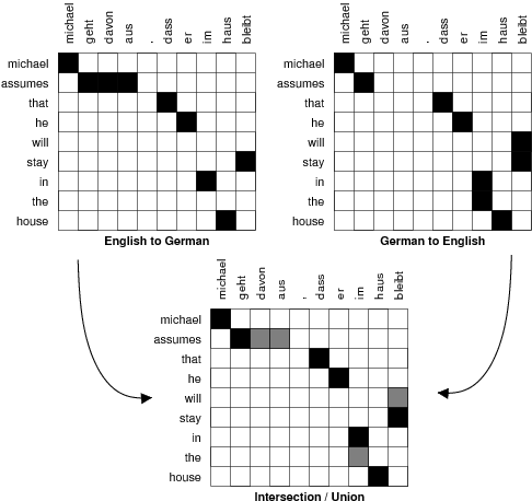
First, the parallel corpus is aligned bidirectionally, e.g., Spanish to English and English to Spanish. This generates two word alignments that have to be reconciled. If we intersect the two alignments, we get a high-precision alignment of high-confidence alignment points. If we take the union of the two alignments, we get a high-recall alignment with additional alignment
points. See the figure below for an illustration.
Researchers differ in their methods where to go from here. We describe the details below.
Methods for Learning Phrase Translations
Most of the recently proposed methods use a word alignment to learn a phrase translation table. We discuss three such methods in this section and one exception.
Marcu and Wong
First, the exception: Marcu and Wong (EMNLP, 2002) proposed to establish phrase correspondences directly in a parallel corpus. To learn such correspondences, they introduced a phrase-based joint probability model that simultaneously generates both the source and target sentences in a parallel corpus.
Expectation Maximization learning in Marcu and Wong's framework yields both (i) a joint probability distribution φ(e, f), which reflects the probability that phrases e and f are translation equivalents; (ii) and a joint distribution d(i,j), which reflects the probability that a phrase at position i is translated into a phrase at position j.
To use this model in the context of our framework, we simply marginalize the joint probabilities estimated by Marcu and Wong (EMNLP, 2002) to conditional probabilities. Note that this approach is consistent with the approach taken by Marcu and Wong themselves, who use conditional models during decoding.
Och and Ney
Och and Ney (Computational Linguistics, 2003) propose a heuristic approach to refine the alignments obtained from GIZA++. At a minimum, all alignment points of the intersection of the two alignments are maintained. At a maximum, the points of the union of the two alignments are considered. To illustrate this, see the figure below. The intersection points are black, the additional points in the union are shaded grey.
Och and Ney explore the space between intersection and union with expansion heuristics
that start with the intersection and add additional alignment points. The decision which points to add may depend on a number of criteria:
- In which alignment does the potential alignment point exist? Foreign-English or English-foreign?
- Does the potential point neighbor already established points?
- Does neighboring mean directly adjacent (block-distance), or also diagonally adjacent?
- Is the English or the foreign word that the potential point connects unaligned so far? Are both unaligned?
- What is the lexical probability for the potential point?
Och and Ney (Computational Linguistics, 2003) are ambigous in their description about which alignment points are added in their refined method. We reimplemented their method for Moses, so we will describe this interpretation here.
Our heuristic proceeds as follows: We start with intersection of the two word alignments. We only add new alignment points that exist in the union of two word alignments. We also always require that a new alignment point connects at least one previously unaligned word.
First, we expand to only directly adjacent alignment points. We check for potential points starting from the top right corner of the alignment matrix, checking for alignment points for the first English word, then continue with alignment points for the second English word, and so on.
This is done iteratively until no alignment point can be added anymore. In a final step, we add non-adjacent alignment points, with otherwise the same requirements.
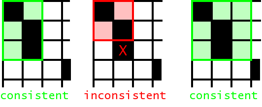
We collect all aligned phrase pairs that are consistent with the word alignment: The words in a legal phrase pair are only aligned to each other, and not to words outside. The set of bilingual phrases BP can be defined formally (Zens, KI 2002) as:
BP(f1J,e1J,A) = { ( fjj+m,eii+n ) }: forall (i',j') in A : j <= j' <= j+m <-> i <= i' <= i+n
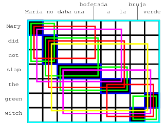
See the figure below for some examples what this means. All alignment points for words that are part of the phrase pair have to be in the phrase alignment box. It is fine to have unaligned words in a phrase alignment, even at the boundary.
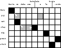
The figure below displays all the phrase pairs that are collected according to this definition for the alignment from our running example.
(Maria, Mary),
(no, did not),
(slap, daba una bofetada),
(a la, the),
(bruja, witch),
(verde, green),
(Maria no, Mary did not),
(no daba una bofetada, did not slap),
(daba una bofetada a la, slap the),
(bruja verde, green witch),
(Maria no daba una bofetada, Mary did not slap),
(no daba una bofetada a la, did not slap the),
(a la bruja verde, the green witch)
(Maria no daba una bofetada a la, Mary did not slap the),
(daba una bofetada a la bruja verde, slap the green witch),
(no daba una bofetada a la bruja verde, did not slap the green witch),
(Maria no daba una bofetada a la bruja verde, Mary did not slap the green witch)
Given the collected phrase pairs, we estimate the phrase translation probability distribution by relative frequency: φ(f|e) = count(f,e) Σf count(f,e)
No smoothing is performed, although lexical weighting addresses the problem of sparse data. For more details, see our paper on phrase-based translation (Koehn at al, HLT-NAACL 2003).
Tillmann
Tillmann (EMNLP, 2003) proposes a variation of this method. He starts with phrase alignments based on the intersection of the two GIZA++ alignments and uses points of the union to expand these. See his presentation for details.
Venugopal, Zhang, and Vogel
Venugopal et al. (ACL 2003) allows also for the collection of phrase pairs that are violated by the word alignment. They introduce a number of scoring methods take consistency with the word alignment, lexical translation probabilities, phrase length, etc. into account.
Zhang et al. (2003) proposes a phrase alignment method that is based on word alignments and tries to find a unique segmentation of the sentence pair, as it is done by Marcu and Wong directly. This enables them to estimate joint probability distributions, which can be marginalized into conditional probability distributions.
Vogel et al. (2003) reviews these two methods and shows that the combining phrase tables generated by different methods improves results.
Decoder
This section describes the Moses decoder from a more theoretical perspective. The decoder was originally developed for the phrase model proposed by Marcu and Wong. At that time, only a greedy hill-climbing decoder was available, which was unsufficent for our work on noun phrase translation (Koehn, PhD, 2003).
The decoder implements a beam search and is roughly similar to work by Tillmann (PhD, 2001) and Och (PhD, 2002). In fact, by reframing Och's alignment template model as a phrase translation model, the decoder is also suitable for his model, as well as other recently proposed phrase models.
We start this section with defining the concept of translation options, describe the basic mechanism of beam search, and its neccessary components: pruning, future cost estimates. We conclude with background on n-best list generation.
Translation Options
Given an input string of words, a number of phrase translations could be applied. We call each such applicable phrase translation a translation option. This is illustrated in the figure below, where a number of phrase translations for the Spanish input sentence Maria no daba uma bofetada a la bruja verde are given.
These translation options are collected before any decoding takes place. This allows a quicker lookup than consulting the whole phrase translation table during decoding. The translation options are stored with the information
- first foreign word covered
- last foreign word covered
- English phrase translation
- phrase translation probability
Note that only the translation options that can be applied to a given input text are necessary for decoding. Since the entire phrase translation table may be too big to fit into memory, we can restrict ourselves to these translation options to overcome such computational concerns. We may even generate a phrase translation table on demand that only includes valid translation options for a given input text. This way, a full phrase translation table (that may be computationally too expensive to produce) may never have to be built.
Core Algorithm
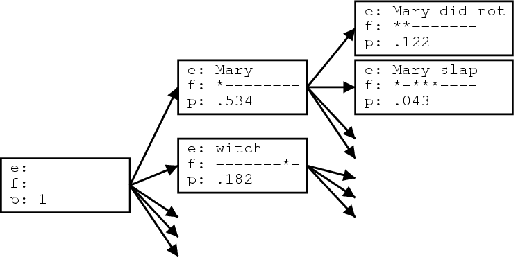
The phrase-based decoder we developed employs a beam search algorithm, similar to the one used by Jelinek (book "Statistical Methods for Speech Recognition", 1998) for speech recognition. The English output sentence is generated left to right in form of hypotheses.
This process illustrated in the figure below. Starting from the initial hypothesis, the first expansion is the foreign word Maria, which is translated as Mary. The foreign word is marked as translated (marked by an asterisk). We may also expand the initial hypothesis by translating the foreign word bruja as witch.
We can generate new hypotheses from these expanded hypotheses. Given the first expanded hypothesis we generate a new hypothesis by translating no with did not. Now the first two foreign words Maria and no are marked as being covered. Following the back pointers of the hypotheses we can read of the (partial) translations of the sentence.
Let us now describe the beam search more formally. We begin the search in an initial state where no foreign input words are translated and no English output words have been generated. New states are created by extending the English output with a phrasal translation of that covers some of the foreign input words not yet translated.
The current cost of the new state is the cost of the original state multiplied with the translation, distortion and language model costs of the added phrasal translation. Note that we use the informal concept cost analogous to probability: A high cost is a low probability.
Each search state (hypothesis) is represented by
- a back link to the best previous state (needed for finding the best translation of the sentence by back-tracking through the search states)
- the foreign words covered so far
- the last two English words generated (needed for computing future language model costs)
- the end of the last foreign phrase covered (needed for computing future distortion costs)
- the last added English phrase (needed for reading the translation from a path of hypotheses)
- the cost so far
- an estimate of the future cost (is precomputed and stored for efficiency reasons, as detailed in below in special section)
Final states in the search are hypotheses that cover all foreign words. Among these the hypothesis with the lowest cost (highest probability) is selected as best translation.
The algorithm described so far can be used for exhaustively searching through all possible translations. In the next sections we will describe how to optimize the search by discarding hypotheses that cannot be part of the path to the best translation. We then introduce the concept of comparable states that allow us to define a beam of good hypotheses and prune out hypotheses that fall out of this beam. In a later section, we will describe how to generate an (approximate) n-best list.
Recombining Hypotheses
Recombining hypothesis is a risk-free way to reduce the search space.
Two hypotheses can be recombined if they agree in
- the foreign words covered so far
- the last two English words generated
- the end of the last foreign phrase covered
If there are two paths that lead to two hypotheses that agree in these properties, we keep only the cheaper hypothesis, e.g., the one with the least cost so far. The other hypothesis cannot be part of the path to the best translation, and we can safely discard it.
Note that the inferior hypothesis can be part of the path to the second best translation. This is important for generating n-best lists.
Beam Search
While the recombination of hypotheses as described above reduces the size of the search space, this is not enough for all but the shortest sentences. Let us estimate how many hypotheses (or, states) are generated during an exhaustive search. Considering the possible values for the properties of unique hypotheses, we can estimate an upper bound for the number of states by N ~ 2nf |Ve|2 nf where nf is the number of foreign words, and |Ve| the size of the English vocabulary. In practice, the number of possible English words for the last two words generated is much smaller than |Ve|2. The main concern is the exponential explosion from the 2nf possible configurations of foreign words covered by a hypothesis. Note this causes the problem of machine translation to become NP-complete (Knight, Computational Linguistics, 1999) and thus dramatically harder than, for instance, speech recognition.
In our beam search we compare the hypotheses that cover the same number of foreign words and prune out the inferior hypotheses. We could base the judgment of what inferior hypotheses are on the cost of each hypothesis so far. However, this is generally a very bad criterion, since it biases the search to first translating the easy part of the sentence. For instance, if there is a three word foreign phrase that easily translates into a common English phrase, this may carry much less cost than translating three words separately into uncommon English words. The search will prefer to start the sentence with the easy part and discount alternatives too early.
So, our measure for pruning out hypotheses in our beam search does not only include the cost so far, but also an estimate of the future cost. This future cost estimation should favor hypotheses that already covered difficult parts of the sentence and have only easy parts left, and discount hypotheses that covered the easy parts first. We describe the details of our future cost estimation in the next section.
Given the cost so far and the future cost estimation, we can prune out hypotheses that fall outside the beam. The beam size can be defined by threshold and histogram pruning. A relative threshold cuts out a hypothesis with a probability less than a factor α of the best hypotheses (e.g., α = 0.001). Histogram pruning keeps a certain number n of hypotheses (e.g., n = 100).
Note that this type of pruning is not risk-free (opposed to the recombination, which we described earlier). If the future cost estimates are inadequate, we may prune out hypotheses on the path to the best scoring translation. In a particular version of beam search, A* search, the future cost estimate is required to be _admissible_, which means that it never overestimates the future cost. Using best-first search and an admissible heuristic allows pruning that is risk-free. In practice, however, this type of pruning does not sufficiently reduce the search space. See more on search in any good Artificial Intelligence text book, such as the one by Russel and Norvig ("Artificial Intelligence: A Modern Approach").
The figure below gives pseudo-code for the algorithm we used for our beam search. For each number of foreign words covered, a hypothesis stack in created. The initial hypothesis is placed in the stack for hypotheses with no foreign words covered. Starting with this hypothesis, new hypotheses are generated by committing to phrasal translations that covered previously unused foreign words. Each derived hypothesis is placed in a stack based on the number of foreign words it covers.
 initialize hypothesisStack[0 .. nf];
 create initial hypothesis hyp_init;
 add to stack hypothesisStack[0];
 for i=0 to nf-1:
   for each hyp in hypothesisStack[i]:
     for each new_hyp that can be derived from hyp:
       nf[new_hyp] = number of foreign words covered by new_hyp;
       add new_hyp to hypothesisStack[nf[new_hyp]];
       prune hypothesisStack[nf[new_hyp]];
 find best hypothesis best_hyp in hypothesisStack[nf];
 output best path that leads to best_hyp;
We proceed through these hypothesis stacks, going through each hypothesis in the stack, deriving new hypotheses for this hypothesis and placing them into the appropriate stack (see figure below for an illustration). After a new hypothesis is placed into a stack, the stack may have to be pruned by threshold or histogram pruning, if it has become too large. In the end, the best hypothesis of the ones that cover all foreign words is the final state of the best translation. We can read off the English words of the translation by following the back links in each hypothesis.
Future Cost Estimation
Recall that for excluding hypotheses from the beam we do not only have to consider the cost so far, but also an estimate of the future cost. While it is possible to calculate the cheapest possible future cost for each hypothesis, this is computationally so expensive that it would defeat the purpose of the beam search.
The future cost is tied to the foreign words that are not yet translated. In the framework of the phrase-based model, not only may single words be translated individually, but also consecutive sequences of words as a phrase.
Each such translation operation carries a translation cost, language model costs, and a distortion cost. For our future cost estimate we consider only translation and language model costs. The language model cost is usually calculated by a trigram language model. However, we do not know the preceding English words for a translation operation. Therefore, we approximate this cost by computing the language model score for the generated English words alone. That means, if only one English word is generated, we take its unigram probability. If two words are generated, we take the unigram probability of the first word and the bigram probability of the second word, and so on.
For a sequence of foreign words multiple overlapping translation options exist. We just described how we calculate the cost for each translation option. The cheapest way to translate the sequence of foreign words includes the cheapest translation options. We approximate the cost for a path through translation options by the product of the cost for each option.
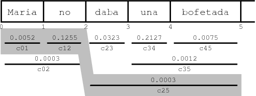
To illustrate this concept, refer to the figure below. The translation options cover different consecutive foreign words and carry an estimated cost cij. The cost of the shaded path through the sequence of translation options is c01c12c25 = 1.9578 * 10-7.
The cheapest path for a sequence of foreign words can be quickly computed with dynamic programming. Also note that if the foreign words not covered so far are two (or more) disconnected sequences of foreign words, the combined cost is simply the product of the costs for each contiguous sequence. Since there are only n(n+1)/2 contiguous sequences for n words, the future cost estimates for these sequences can be easily precomputed and cached for each input sentence. Looking up the future costs for a hypothesis can then be done very quickly by table lookup. This has considerable speed advantages over computing future cost on the fly.
N-Best Lists Generation
Usually, we expect the decoder to give us the best translation for a given input according to the model. But for some applications, we might also be interested in the second best translation, third best translation, and so on.
A common method in speech recognition, that has also emerged in machine translation is to first use a machine translation system such as our decoder as a base model to generate a set of candidate translations for each input sentence. Then, additional features are used to rescore these translations.
An n-best list is one way to represent multiple candidate translations. Such a set of possible translations can also be represented by word graphs (Ueffing et al., EMNLP 2002) or forest structures over parse trees (Langkilde, EACL 2002). These alternative data structures allow for more compact representation of a much larger set of candidates. However, it is much harder to detect and score global properties over such data structures.
Additional Arcs in the Search Graph
Recall the process of state expansions. The generated hypotheses and the expansions that link them form a graph. Paths branch out when there are multiple translation options for a hypothesis from which multiple new hypotheses can be derived. Paths join when hypotheses are recombined.
Usually, when we recombine hypotheses, we simply discard the worse hypothesis, since it cannot possibly be part of the best path through the search graph (in other words, part of the best translation).
But since we are now also interested in the second best translation, we cannot simply discard information about that hypothesis. If we would do this, the search graph would only contain one path for each hypothesis in the last hypothesis stack (which contains hypotheses that cover all foreign words).
If we store information that there are multiple ways to reach a hypothesis, the number of possible paths also multiplies along the path when we traverse backward through the graph.
In order to keep the information about merging paths, we keep a record
of such merges that contains
- identifier of the previous hypothesis
- identifier of the lower-cost hypothesis
- cost from the previous to higher-cost hypothesis
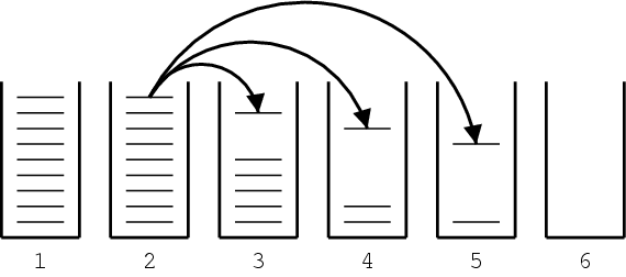
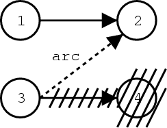
The figure below gives an example for the generation of such an arc: in this case, the hypotheses 2 and 4 are equivalent in respect to the heuristic search, as detailed above. Hence, hypothesis 4 is deleted. But since we want to keep the information about the path leading from hypothesis 3 to 2, we store a record of this arc. The arc also contains the cost added from hypothesis 3 to 4. Note that the cost from hypothesis 1 to hypothesis 2 does not have to be stored, since it can be recomputed from the hypothesis data structures.
Mining the Search Graph for an n-Best List
The graph of the hypothesis space can be also be viewed as a probabilistic finite state automaton. The hypotheses are states, and the records of back-links and the additionally stored arcs are state transitions. The added probability scores when expanding a hypothesis are the costs of the state transitions.
Finding the n-best path in such a probabilistic finite state automaton is a well-studied problem. In our implementation, we store the information about hypotheses, hypothesis transitions, and additional arcs in a file that can be processed by the finite state toolkit Carmel, which we use to mine the n-best lists. This toolkit uses the _n_ shortest paths algorithm by Eppstein (FOCS, 1994).
Our method is related to work by Ueffing (2002) for generating n-best lists for IBM Model 4.

 Language Models